Signal processing and analysis of human brain potentials (EEG) [Exercise 7]
Download dataset
More on the dataset or the original studies. In short: Faces were shown with varying noise added to them (phase-randomization in 2D-fourier space). An example: 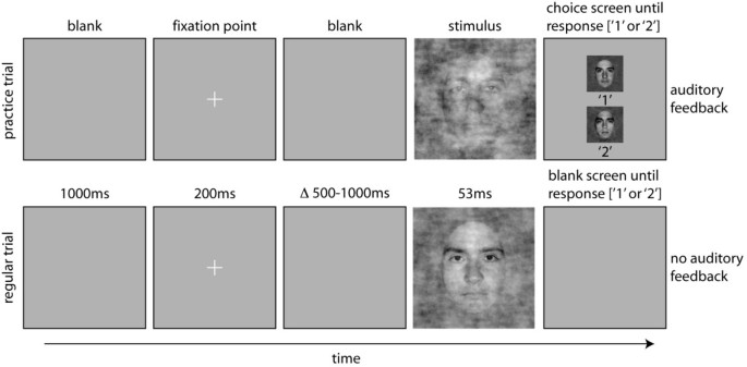
We will build a designmatrix to manually apply a regression model to all timepoints. Then we will do the same thing within MNE!
from mne.datasets.limo import load_data
# choose any subject 1 - 18
limo_epochs = load_data(subject=4,path='../local/limo') #- Extract data from electrode
B11, this will be your ‘y’ - The linear covariate is saved in a dataframe called limo_epochs.metadata. Metadata is yet another way that you can save event-related information besides annotations & events
- Generate a (design) matrix consisting of an intercet and a linear predictor of phase-coherence.
- Use
scipy.linalg.lstsqor similar functions to solve the LeastSquares Problem at each time-point of the epoch - Plot the result parameters and comment what the two parameters represent.
Conditional ERPs
We now have values for an intercept and for a slope, but it is hard to gauge the true meaning of the slope. Therefore we going to generate predicted values at specific levels of the continuous variable. Note that in principle, you could also extrapolate (going outside the range of 0,1) or interpolate (values that were not run in the experiment), but it is not necessary here. These predictions can be seen as conditional ERPs, because you condition on the continuous variable to be a specific value.
- Evaluate the continuous regressor at the unique 18 coherence (noise) levels that were used in the experiment and plot them (hint: you could use \(X_{new}b\) but dont have to in this simple example)
- Should you add the Intercept to the resulting Plot?
Compare it to binned data
- Next, generate one evoked.average() for each of the 18 stimulus coherence values.
- Plot them and compare them to your predictions. How well does a continuous predictor capture the data?
Converting a continuous predictor to a spline predictor
- For this exercise we need
from ccs_eeg_utils import spline_matrixfunction. - The function requires to specify where the spline bases should be evaluated
x(the coherence value of each epoch) and where theknotsshould be. Think of the knots as the anchorpoints of the spline set. (Note: There is a huge literature on knot placement etc. we just use a linspace over the range of our continuous variable. If you want you can play around and e.g. place more knots in the middle than the end). How many knots you ask? Choose a reasonable low number, you can change it later again. There are ways to decide this but they are outside the tutorial. Stay below 10. - Plot the basisfunction as line-plots
- Plot the designmatrix as an 2D image
- Fit the splines to your data (Note: If you wonder about the intercept, there are two ways here.Take the whole spline matrix and dont add an intercept {the intercept is implicit in the spline matrix}, or remove one spline and add an intercept {now all spline-predictors are relativ to the intercept}. Note that due to potential asymmetries in the spline basis set, the intercept is not necessarily what you would expect, see below)
- Plot the resulting “raw” coefficients
- The “raw” coefficients are hard to interpret. We should run conditional values again. Evaluate the fitted spline-betas at the respective 18 coherence levels and plot them.
Add another predictor
- We will add a categorical regressor to our spline designmatrix: The difference of FaceA vs. FaceB. Note: If you havent remove a spline-column yet, please do so now and include an intercept.
- Because it is a categorical predictor, we have to encode it using either dummy coding (e.g. FaceA = 0, FaceB = 1) or effect coding (FaceA = -0.5, FaceB = 0.5 {you could also use -1 / 1})
- Fit the model, and plot the faceA/faceB effect
- In order to facilitate calculating such effects, often a contrast-vector (or matrix) is used. We have a vector \(b\) that in our case represents \([b_{intercept},b_{faceB},b_{spline1}, \ddots, b_{splineN}]\). We typically want to use a sum of predictors, ie. \(b_{intercept}\) + \(b_{faceB}\) which can be represented as a matrix multiplication of \(b*c\) with \(c = [1,1,0,\dots,0]\). If we chose effect coding before, we would need to put in the effect coded coefficients in our contrast-vector. I.e. \(c = [1,-0.5,0,\dots,0]\) or \(c = [1,-1,0,\dots,0]\). And finally, we could also combine multiple contrast vectors to one matrix to evaluate multiple effects of interest.
- Use a contrast matrix to plot the FaceA and FaceB ERP. Note that in difference to the example contrats-vector above, we now also want to add the correct spline-values. For this evaluate the spline-coefficients at noise-coherence of 0.9 and replace the 0’s of your \(c_{spline1} \dots c_{splineN}\) contrast vector.
Bonus:
- There could be an interaction between the spline set and the categorical variable. For this, we have to calculate all pairwise multiplications of the faceB-column, with the spline columns.
- Fit the resulting model and check whether you found an interaction effect
Fitting a model in MNE
Typically, one wouldnt fit the models with scipy manually, but one can use MNE to handle the fits (or even dedicated toolboxes like unfold* - but I am not aware of a documented toolbox in python). This also gives you much more support, i.e. gives you standard errors(=SE),and through t = effect/SE, the t-values which can be easily looked up in the analytical H0 distribution and converted to single subject p-values.
import
from mne.stats import linear_regressionFit a model
y~1 + faceB + coherence, thus a model with linear coherence effect: mne also requires to specify your own designmatrix, you can also give the columns names usingres = linear_regression(...,names=['Intercept','effectB' ...]).You can access the terms using res[‘Intercept’], and plot e.g. the betas using
res['Intecept'].beta.plot()Because we have all channels now, we can also plot topoplots. Think about how you could visualize the splines as topoplots (note: this is a hard question)
You can also plot the p-values using res[‘phase_coherence’].p_val.plot(). Do they follow your intuition?
Bonus: What does the distribution (histogram) of p-values of phase-coherence look like during the baseline? (note, bad channels are not automatically removed in MNE, thus you might want to increase your bin-width to spot them
Schleichwerbung ;-)